Introduction to measurements and statistics for shooters

Random Universe

Our world is random. When anything is measured with sufficient level of precision several times, the results are usually slightly different. Why?

Every physical object consists of a huge number of tiny particles - atoms, molecules - that are moving (flying in gas or in liquid, or vibrating in solid bodies) under the influence of heat. Heat itself is but a measure of this internal movement. The physical parameters of the body (length, temperature, weight) are determined in part by this microscopic dance of its molecules and the similar movement of the the surroundings. The effects of this dance vary in time, which leads to the slight jitter of the body's parameters.

Furthermore, the measuring devices are physical bodies which are susceptible to similar jitter, which adds another degree of randomness to the measurements. Because precise instruments amplify the value to measure it, the random jitter within the instruments themselves is also amplified, often disproportionately.

This randomness is not always perceptible because our measurements are typically very coarse. Occasionally, however, it gets they get magnified and can be easily observable. Shooting is one activity especially amenable to such amplification of randomness, because even the slightest variability leads to large differences over the long distance.

In probability and statistics, a random variable is a variable whose value is subject to variations due to chance. Every physical parameter that we can measure - weight, length, temperature - are random variables.

How do you measure randomness?

Let's say you have a precise scale and a bullet. You put the bullet on the scale, and the reading is 167.991 grain. What is the weight of the bullet?

The obvious answer is that it is 167.991 grains, right?

Well, but what if you weigh it again and now the scale says 168.053? We repeat the weighing several more times and get the following results:

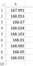
What now? There is no single number, but there is still plenty of information. For instance, we can say that all numbers lie between 167.991 and 168.103.

Or we can say that with the probability of 95% another measurement would fall in between 167.98 and 168.11 (how we got to this statement is explained below).

Most of the information we have about the world that surrounds us really exists as a bunch of confidence intervals (we are 95% certain that the radius of Earth is between X and Y meters). 95% is actually a commonly accepted confidence interval in business and sometimes in engineering - we consider that we know something pretty well if we are 95% certain that it is true. In science, however, the requirements are much stronger - we want to be 99.5% certain before we declare something as a scientific fact.

Probability distribution

But is the confidence interval enough? Consider the following two sets of measurements:

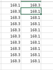
The measurements all fall into the same interval. But it seems intuitive that the physical bodies in these two experiments are different.

Probability distribution assigns a probability to each of the possible outcomes of a random experiment.

Whether expressed as a graph or a formula, it will tell you how likely one is to get a particular value upon the measurement.

Standard deviation (σ)

Another important measure of randomness is the standard deviation. For a series of measurements the standard deviation shows how far an "average measurement" is from the average of all measurements. If the standard deviation is small, you should have good confidence in the measurement (there is a high likelihood that subsequent measurements will yield similar results - or subsequent shots will land near the target).

If you have N measurements x1, x2, ..., xN, then the standard deviation is

For example, let's say you shoot 10 rounds at a bulls eye, and the vertical distribution of the shots is as follows (0 is the target, positive axis points up):

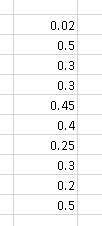
The average deflection is 0.32, and the standard deviation is 0.14.

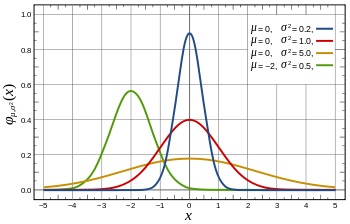
Normal distribution

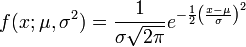
One of the most famous functions in mathematics is the so called "bell curve", or normal distribution. It is so famous because almost every physical event is described by it. The reason for it is the Central Limit Theorem, my favorite result in statistics.

Central Limit Theorem states that, given certain conditions, the mean of a sufficiently large number of independent random variables, each with finite mean and variance, will be approximately normally distributed.

Because every physical thing that surrounds us is a combination of many things, and its properties are influenced by many random factors, the net result of all these influences end up being normally distributed, even if the individual factors are not.

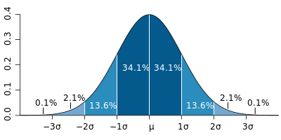
A normally distributed value has a 95% confidence interval of (roughly) +/- 2σ

If we know that the distribution is normal (and it almost always is), and we can estimate its standard deviation, we can predict subsequent results with a level of confidence.

Estimating the parameters of the normal distribution

If you have a bunch of results, you can compute the standard deviation of these results, and then the confidence interval for the future behavior.

It is important to understand, however, that what you compute based on limited number of experiments, is just an estimate of what these parameters might be. To illustrate this, let's see you've made fifty shots at the target and recorded the vertical dispersion as follows:

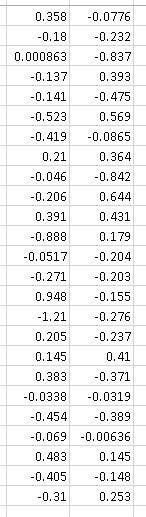
The average vertical POI from this sample is -0.07, and the standard deviation is 0.41. Looking good so far? Well, if you were to shoot only 25 times, your average would have been -0.09, and your standard deviation 0.44. Out of 10-shot sample, you would have worked out -0.11 average and 0.28 standard deviation, and out of 5-shot sample, -0.02 and 0.20, respectively.

The "true" standard deviation of the sample above is actually 0.5 (this is how I generated it). Because we only ran finite number of experiment, we have arrived at a series of estimates for the parameters of the distribution, but not the real values. The more experiments we run, the more the results will fill the real curve, and the closer we will get to the true value.

It turns out, however, that we can do pretty good estimates even using finite number of experiments. Standard deviation has its own distribution, called Student's t-distribution. The mathematics of it is far too complicated to explain here, but there is a handy function in Excel - STDEV.S - that estimates the real value of σ from a finite set of measured values.

Are they different?

If you can estimate the confidence intervals, you can answer many really interesting question about your data. For example, given the two data sets, are they statistically different?

For example, let's go back to our previous example, and ask ourselves whether the first column is materially different from the second one.

Perhaps you varied powder a little, and want to know whether it resulted in a vertical shift of the point of impact.

On the surface, the average of the first column is -0.09, and for the second it is -0.05, so there might be a difference. However, the confidence interval for the first column is (+/- 2σ) from -0.97 to 0.79, and for the second, -0.82 to 0.72. Not only both values are well within each other's confidence intervals, but even the intervals themselves significantly overlap!

The difference between two values is considered to be statistically significant, if they lie outside each other's confidence intervals. So to determine this mathematically, you can compute the confidence intervals of the two datasets, and make sure that their averages lie outside each others' confidence intervals.

Note, however, that the confidence intervals may be very wide if you did not run enough experiments. So it could be that the values look the same only because you did not collect sufficient stats.

Here is how to determine if two sequences of numbers are statistically different in Excel.

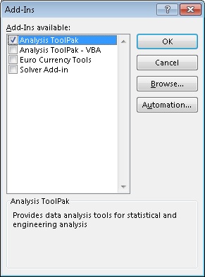
First, you need to enable Data Analysis Add in: go to Options -> Add-Ins, and click on "Go..."

In the dialog that opens you will need to check Analysis Toolpack.

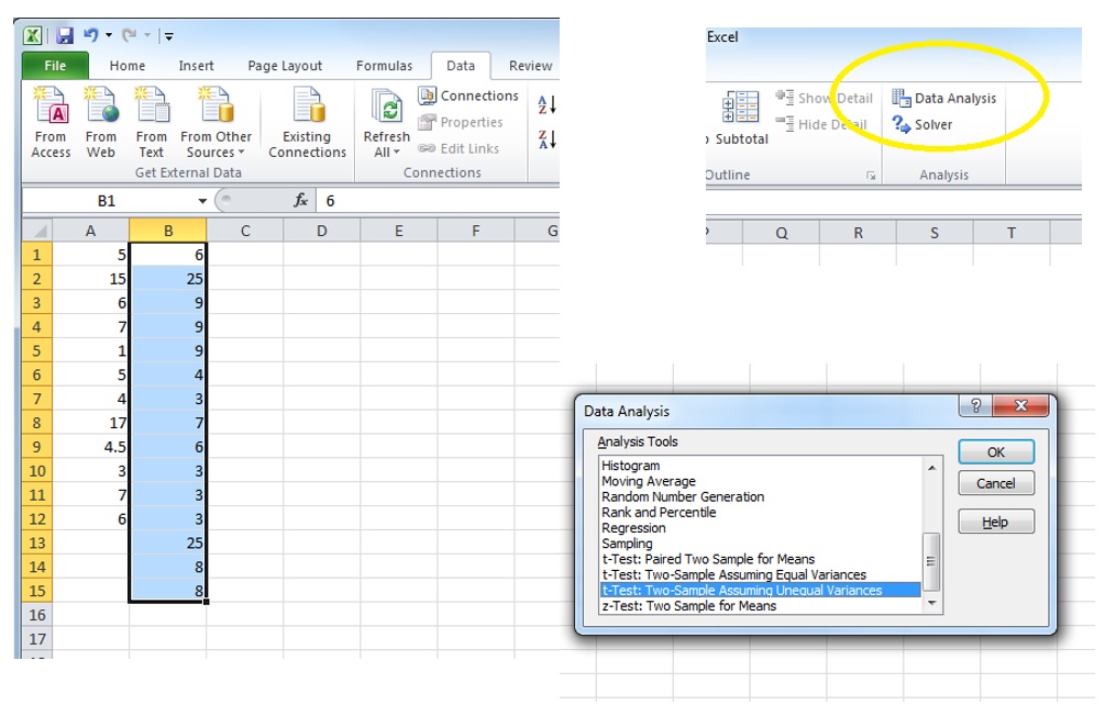
You should then see "Data Analysis" option in your Data tab. You can now click on it and choose "t-Test: Two-Sample Assuming Unequal Variances".

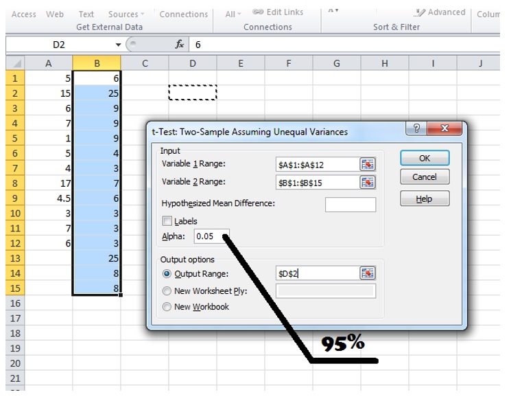
Put the ranges for the two datasets in the variable inputs, and ensure that Alpha is 0.05, which corresponds to 95% confidence level interval.

Clicking OK produces the following output:

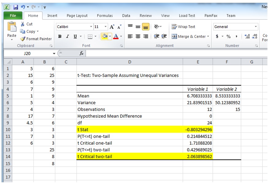
Note two values: t-stat and t-critical. If your t-sta's absolute value (dropping the sign if it is negative) is below t-critical value, the difference is not statistically significant.